lafarren.com
Image Completion
Overview
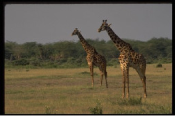
Input image of giraffes with a black border.
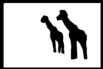
Mask image. Black regions will be filled by the algorithm.
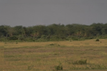
The completed image.
This code is based on a paper titled ![]() Image Completion Using Efficient Belief Propagation via Priority Scheduling and Dynamic Pruning, by
Nikos Komodakis and
Georgios Tziritas.
Given an image with missing regions, an image completion algorithm attempts to fill the missing regions such that a visually coherent
result is achieved. There are many
approaches to the problem, and in mid-2009 I stumbled upon Komodakis's and Tziritas's research, and was impressed at the quality of the results
(see pages 23 and 24 of the
PDF).
Image Completion Using Efficient Belief Propagation via Priority Scheduling and Dynamic Pruning, by
Nikos Komodakis and
Georgios Tziritas.
Given an image with missing regions, an image completion algorithm attempts to fill the missing regions such that a visually coherent
result is achieved. There are many
approaches to the problem, and in mid-2009 I stumbled upon Komodakis's and Tziritas's research, and was impressed at the quality of the results
(see pages 23 and 24 of the
PDF).
When I began implementing their research I had planned on releasing it as a Photoshop plugin. But after a month of coding, I saw the work that Adobe was incorporating into their then-upcoming Photoshop CS5, and knew I couldn't compete with them. Their technique was faster, more flexible, and built right into the application. Rather than let this code go to waste, it seemed better to release it under the GPL, with hopes that someone will find it useful or educational.
How It Works
The paper contains the full level of detail, but what follows is a quick, high level description of how the algorithm works. The approach uses data from the known region of the image - that is, the part of the image that isn't missing - to fill the unknown region. It does this by first creating a lattice (i.e., a grid) over the image where each point, or node, is a fixed width and height from its four immediate neighbors - the nodes above, below, left, and right. Then, it builds a set of all possible rectangles of pixel data from the known region. A given rectangle of known pixel data is called a patch (the paper also refers to them as labels, a nod to the research's roots in Markov Random Fields and Belief Propagation). Each patch is twice the width and height of the space between each lattice node. Eventually, the lattice's nodes are what the centers of the chosen patches hang on when filling the unknown region, and because patches are twice the size as the lattice's gaps, each patch overlaps with the patches of its immediate four neighbors, as well as its four diagonal neighbors. See figures 5 and 6 of the PDF (pages 7 and 8).
The meat of the algorithm determines which patches to use at each lattice node. First, at a given node, it scores how agreeably each patch overlaps with the known pixel data. It does this by calculating an energy value, which is simply the sum of the squared differences of each overlapping pixels' RGB components. The more similar the pixels are, the lower the difference in color, and thus a lower energy between the patch and the known pixels at that node. Nodes toward the interior of the unknown region may have patches that don't overlap the known region at all, and therefore the energies for each patch at those points will be zero. This initial pass determines the confidence level of each node by measuring the separation in energy scores for all its patches. Nodes that overlap a lot of known pixels will tend to have some agreeable patches and some not-so-agreeable patches, especially if the known pixel data contains unique, non-uniform features. For example, consider the image below of a ship. Given the uniformity of the sky and ocean regions, the nodes within those regions have many patches that are good, coherent candidates. On the other hand, nodes that overlap the horizon have fewer patches that will agree with the horizon's sharp bisection, leading to fewer good candidates at those nodes. This high separation between low and high energy scores increases the algorithm's confidence in the horizon nodes. If an interior node doesn't overlap with any known pixels, then it won't have any separation in energy scores, because every patch will yield zero energy. Such nodes are considered low-confidence after the first pass. By interpreting fewer "good" candidate patches as a positive thing, the algorithm uses those nodes as anchors of certainty from which to proceed.
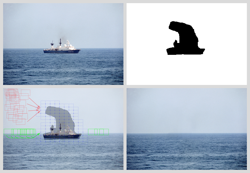
An image of a ship, the image completion mask, and the result. The lower left image provides a glimpse into the image completion process. The lattice is shown in the form of a light blue grid, with lattice nodes shown as blue dots. Nearly any sky patch (in red) is a good candidate for a sky node, while a horizon node has many times fewer good candidate patches to use (in green). Because horizon nodes have a narrower, more focused possibility set, the algorithm has higher confidence in evaluating those nodes first.
After the initial node confidences are calculated, the algorithm takes two passes over the nodes. The first pass, called the forward pass, steps through the nodes in order of highest-to-lowest confidence. For the current node, it prunes most of its potential patches, retaining only a small set of low energy patches. Then, it sends energy messages from the current node to each of the node's immediate neighbors, but only if the neighbor hasn't been visited yet during the forward pass. Each message communicates how agreeable one of the node's patches is with one of the neighbor's patches. It sends one message per patch pairing, for all of the current node's patches, against all of the neighbor's patches. For example, if the current node is A, which has a post-pruned set of Ap = {A's patches}, and one of A's neighbors is node B, which has Bp = {B's patches}, then A tests how well every patch in Ap overlaps with every patch in Bp when those patches are positioned at the nodes' coordinates. After all messages are sent in the forward pass, the backward pass occurs, which steps through the nodes in reverse order of the forward pass, and calculates and sends messages from the current node to its neighbors in the opposite direction. This flow of information through the graph is crucial for globally optimizing which patches fit well together. Messages are also the sole means of finding the patches for a fully interior node - that is, a node that doesn't overlap any known pixel data. Incoming message values from neighboring nodes are also used to update the receiving node's confidence.
After several passes, the messages typically stabilize and a solution is found. At each node, the patch with the lowest combined energy (known pixel overlap + messages) is what ought to be used at that node's position. Those patches are composited into the original image, and the result is written to an output image.
Limitations and Room For Improvement
Elephant image completion input, mask, and result.
In order to produce decent results, the input image's known region must have good source data that the algorithm can use to fill the unknown region. It seems to work best with images containing natural subject matter, or very regularly patterned images. It doesn't work well when filling a very specific missing subject, such as the parts of a face, because the algorithm has no notion of an image's high level context.
The compositors I wrote can be improved upon... a lot. The normal patch type compositor attempts to soft-blend the edges of each patch, but
the results still have noticeable horizontal and vertical seams, and can sometimes appear over-blurred due to the blending. Adding
a curve matching solution, like that mentioned on page 27 of the
PDF,
would improve the results. I added a ![]() Poisson
based patch type compositor, which helps with seams and improves color-matching, but it still produces rather blurry results.
Poisson
based patch type compositor, which helps with seams and improves color-matching, but it still produces rather blurry results.
Execution speed is a major concern for this algorithm. Given the sheer number of patch energy calculations that must occur, and the fact that the number of calculations increases exponentially with image size, it could take hours or days to solve a large image. To help improve performance, the per-pixel energy calculator parallelizes a batch over multiple hardware threads if the host machine has multiple cores. There's also the settings-low-res-passes=auto command line option, which instructs the program to internally scale an image down to a quickly solvable resolution, and uses the solution found at the lower resolutions to prune patches at each lattice node in the higher resolutions, thus speeding up execution manyfold. The drawback of this approach is that data is lost when downsampling an image, and any error introduced at lower resolutions will propagate to higher resolutions. Still, this option provides a good test result.
Lastly, pages 27 and 28 of the
PDF
suggest transforming the image data to the frequency domain using the
Fast Fourier transform (FFT), performing a
convolution, and using a Windowed Sum Squared Table to calculate the energy between
a single patch and all other patches in logarithmic time. This suggestion is based on a paper titled
![]() Full Search Content Independent Block Matching Based On The Fast Fourier Transform. I implemented an FFT energy calculator
alongside the per-pixel energy calculator,
and at runtime, the code measures the performance between the two calculators for identically sized batches. If uses that profiling data to
choose the faster calculator for future batches. In general, the per-pixel energy calculator works well for smaller images, while the FFT
calculator is better for larger images. Note that Time.cpp
contains a high resolution timer for Windows only, and for other platforms, it falls back on clock() / CLOCKS_PER_SEC.
If you implement a custom high resolution Timer for your platform, I'd be happy to merge it into the master branch; just send a GitHub pull request.
Full Search Content Independent Block Matching Based On The Fast Fourier Transform. I implemented an FFT energy calculator
alongside the per-pixel energy calculator,
and at runtime, the code measures the performance between the two calculators for identically sized batches. If uses that profiling data to
choose the faster calculator for future batches. In general, the per-pixel energy calculator works well for smaller images, while the FFT
calculator is better for larger images. Note that Time.cpp
contains a high resolution timer for Windows only, and for other platforms, it falls back on clock() / CLOCKS_PER_SEC.
If you implement a custom high resolution Timer for your platform, I'd be happy to merge it into the master branch; just send a GitHub pull request.
Code
Git repository:
git://github.com/darrenlafreniere/lafarren-image-completer.git
Or, browse the codebase at github.
Developed using:
- Visual C++ Express 2010
- wxWidgets (2.9, static C runtime (/MT))
- FFTW (3.2.2, static C runtime (/MT), enable single precision)
- Eigen 3.0.0 and UMFPACK (for the Poisson solver)
Thanks to David Doria for getting the Linux/gcc/CMake port running!
If you encounter any problems, please contact me. It's always useful getting more test data to kill the bugs.